It looks like you're using an Ad Blocker.
Please white-list or disable AboveTopSecret.com in your ad-blocking tool.
Thank you.
Some features of ATS will be disabled while you continue to use an ad-blocker.

How to estimate the size and the distance of a UFO?
page: 17
share:
This recurring question is often a source of debate and questions regarding UFOs.
I propose here to better understand the circumstances in which these estimates are possible and, if they are, to provide tools that can give good approximations.
I'll try to be as educational as possible. In addition, I will illustrate my point with a well known photographic case.
I'm also fully open to any idea, opinion or criticism regarding my methodology, in order to improve it.
----------------------------------------------------------------------------------------------
At first, let's talk about theory! For those who do not like maths/geometry, you can directly scroll down to the "Practical Analysis Methodology" chapter, where it's somewhat more fun!
Parameters that may be measured from a photo are expressed in two domains: geometric and radiometric.
Geometric parameters – angles, sizes or distances – make use of pixel positions, in rows and columns, while radiometric parameters are calculated from pixel luminance levels.
Geometric parameters
Photography is based on a principle of conical projection and time integration, which permits representation by a 2-dimensional image of information that occupies a 4-dimensional space (elevation, azimuth, depth and time). It is therefore impossible to reconstruct the whole geometry of a scene from a single photo, except if additional information is available (such as other photos shot from another direction, or data from other sources).
In particular, if the position of pixels in a photo allows (provided other indispensable technical data are available) the calculation of the angular dimensions of an object, an assessment of its real dimensions is only possible if the distance between that object and the camera at shooting time is known or may be estimated.
We shall deal successively with angular distance of a given point from the line of sight (often referred to as the principal axis), and with mensuration of an angular dimension of an object. Then, after a reminder on how to derive a linear dimension from that and from the distance to the lens, we shall review different ways to assess that distance or, at least, a range of possible values.
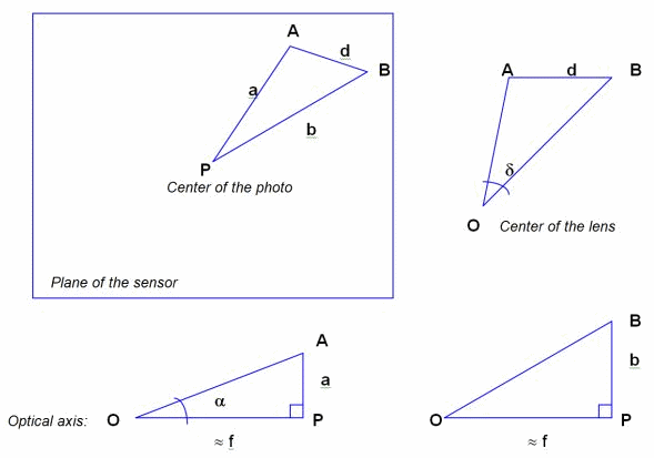
In order to calculate the angular distance from the line of sight, of a point of the scene represented by point A on the sensor, or the angular distance δ between 2 points of the scene represented by points A and B on the sensor, one needs several geometric data: focal length f used for the shot, and distances d, a and b, measured on the photosensitive medium (silver film or CCD array), defined as follows:
f : focal length
a : measure of distance PA on the sensitive medium
b : measure of distance PB on the sensitive medium
d : measure of distance AB on the sensitive medium
O : optical center of the lens
P : center of the photo on the sensitive medium.
Angular localization of an object in the scene
Inside the solid angle defining the camera angular field at shooting time (i.e. the frame of the scene), it is straightforward to determine the angular distance α of a given point A of the image from the line of sight.
In certain cases it will be possible, using additional data, to derive an altitude estimate, if the line of sight is known, and in particular if it is nearly horizontal.
Angular dimensions of an object
Supposing the distance between the points of interest in the scene and the camera is significantly larger than the focal length (which is always true in practice, with the exception of macrophotography), one may assume the following approximation:
Putting into practice, on triangle OAB, the generalized Pythagoras’ theorem, one may calculate the angular size of the object δ between points A and B, with the following formula:
[align=center]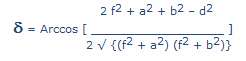 [/align]
Dimensions of an object
To be able to measure – or estimate – the dimension D of an object in a given direction, perpendicular to the line of sight, one must previously know the value – or the estimated value – of 2 pieces of data: the angular dimension δ of the object in that direction and the distance x between that object and the lens.
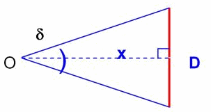
The applicable relation is then:
Estimate of the object’s distance
The distance between an object under study and the lens can of course not be directly derived from the photo, but different analytic approaches can allow an estimate to be made, or at least limits for possible values to be set.
Estimate from other identified and localized objects
If the configuration of elements of the scene allows verification that the distance between the lens and the object under study was compatible to known or measurable limits in its vicinity, one may easily derive a range of possible dimensions for that object, from its angular dimensions.
Depending on cases, reference objects may be buildings, clouds, vegetation or vehicles, etc.
Exploitation of cast shadow
If the object under study casts a shadow visible on the photo, one may try to extract geometric information, in particular if the light source position (the sun is most cases) may be determined in the scene, or if shadows of other objects in that scene may also be brought out.
Analysis of the depth of field
The depth of field defines a range of distance between the lens and an object inside which a photo is sharp (outside movement blur). Therefore it indicates, if the object does appear sharp, possible distance limits between that object and the lens.
This parameter sometimes allows to bring into evidence any incompatibility between sharpness – or blurredness – of an object’s contours on one hand, and its supposed distance from the lens on the other hand (example of « orbs »).
When focus has been set to infinity, which is the case for most photos taken from a digital camera, the depth of field spreads from the hyperfocal distance to infinity. In that case, only objects that are « too close » to the lens may be outside the depth of field, and thus blurred for that reason.
Hyperfocal distance H is calculated as follows:
f : focal length
n : f-number
e : circle of confusion or acceptable sharpness.
Note: I usually use this online DOF calculator that have a large range of cameras in its database and that gives really accurate results for these data.
Parameter "e" is rather subjective by nature. In practice, one assigns a value around 0,03 mm in silver photography and, for a digital camera, a value equal to the size of 2 pixels (generally in the order of 0,01 to 0,02 mm).
If focusing has been done on an object located at a distance D, depth of field limits may be calculated as follows:
PdC : depth of field
Da : front distance (lower limit of the depth of field)
Dp : back distance (upper limit of the depth of field)
I propose here to better understand the circumstances in which these estimates are possible and, if they are, to provide tools that can give good approximations.
I'll try to be as educational as possible. In addition, I will illustrate my point with a well known photographic case.
I'm also fully open to any idea, opinion or criticism regarding my methodology, in order to improve it.
----------------------------------------------------------------------------------------------
At first, let's talk about theory! For those who do not like maths/geometry, you can directly scroll down to the "Practical Analysis Methodology" chapter, where it's somewhat more fun!
MEASURABLE PARAMETERS ON A PHOTO
Parameters that may be measured from a photo are expressed in two domains: geometric and radiometric.
Geometric parameters – angles, sizes or distances – make use of pixel positions, in rows and columns, while radiometric parameters are calculated from pixel luminance levels.
Geometric parameters
Photography is based on a principle of conical projection and time integration, which permits representation by a 2-dimensional image of information that occupies a 4-dimensional space (elevation, azimuth, depth and time). It is therefore impossible to reconstruct the whole geometry of a scene from a single photo, except if additional information is available (such as other photos shot from another direction, or data from other sources).
In particular, if the position of pixels in a photo allows (provided other indispensable technical data are available) the calculation of the angular dimensions of an object, an assessment of its real dimensions is only possible if the distance between that object and the camera at shooting time is known or may be estimated.
We shall deal successively with angular distance of a given point from the line of sight (often referred to as the principal axis), and with mensuration of an angular dimension of an object. Then, after a reminder on how to derive a linear dimension from that and from the distance to the lens, we shall review different ways to assess that distance or, at least, a range of possible values.
In order to calculate the angular distance from the line of sight, of a point of the scene represented by point A on the sensor, or the angular distance δ between 2 points of the scene represented by points A and B on the sensor, one needs several geometric data: focal length f used for the shot, and distances d, a and b, measured on the photosensitive medium (silver film or CCD array), defined as follows:
f : focal length
a : measure of distance PA on the sensitive medium
b : measure of distance PB on the sensitive medium
d : measure of distance AB on the sensitive medium
O : optical center of the lens
P : center of the photo on the sensitive medium.
Angular localization of an object in the scene
Inside the solid angle defining the camera angular field at shooting time (i.e. the frame of the scene), it is straightforward to determine the angular distance α of a given point A of the image from the line of sight.
α = arctan (a/f)
In certain cases it will be possible, using additional data, to derive an altitude estimate, if the line of sight is known, and in particular if it is nearly horizontal.
Angular dimensions of an object
Supposing the distance between the points of interest in the scene and the camera is significantly larger than the focal length (which is always true in practice, with the exception of macrophotography), one may assume the following approximation:
OP ≈ f
Putting into practice, on triangle OAB, the generalized Pythagoras’ theorem, one may calculate the angular size of the object δ between points A and B, with the following formula:
[align=center]
Dimensions of an object
To be able to measure – or estimate – the dimension D of an object in a given direction, perpendicular to the line of sight, one must previously know the value – or the estimated value – of 2 pieces of data: the angular dimension δ of the object in that direction and the distance x between that object and the lens.
The applicable relation is then:
D = 2x x tan (δ/2)
Estimate of the object’s distance
The distance between an object under study and the lens can of course not be directly derived from the photo, but different analytic approaches can allow an estimate to be made, or at least limits for possible values to be set.
Estimate from other identified and localized objects
If the configuration of elements of the scene allows verification that the distance between the lens and the object under study was compatible to known or measurable limits in its vicinity, one may easily derive a range of possible dimensions for that object, from its angular dimensions.
Depending on cases, reference objects may be buildings, clouds, vegetation or vehicles, etc.
Exploitation of cast shadow
If the object under study casts a shadow visible on the photo, one may try to extract geometric information, in particular if the light source position (the sun is most cases) may be determined in the scene, or if shadows of other objects in that scene may also be brought out.
Analysis of the depth of field
The depth of field defines a range of distance between the lens and an object inside which a photo is sharp (outside movement blur). Therefore it indicates, if the object does appear sharp, possible distance limits between that object and the lens.
This parameter sometimes allows to bring into evidence any incompatibility between sharpness – or blurredness – of an object’s contours on one hand, and its supposed distance from the lens on the other hand (example of « orbs »).
When focus has been set to infinity, which is the case for most photos taken from a digital camera, the depth of field spreads from the hyperfocal distance to infinity. In that case, only objects that are « too close » to the lens may be outside the depth of field, and thus blurred for that reason.
Hyperfocal distance H is calculated as follows:
H = f2 / (n x e)
f : focal length
n : f-number
e : circle of confusion or acceptable sharpness.
Note: I usually use this online DOF calculator that have a large range of cameras in its database and that gives really accurate results for these data.
Parameter "e" is rather subjective by nature. In practice, one assigns a value around 0,03 mm in silver photography and, for a digital camera, a value equal to the size of 2 pixels (generally in the order of 0,01 to 0,02 mm).
If focusing has been done on an object located at a distance D, depth of field limits may be calculated as follows:
PdC = Dp – Da
Da = (H x D) / (H + D)
Dp = (H x D) / (H – D)
PdC : depth of field
Da : front distance (lower limit of the depth of field)
Dp : back distance (upper limit of the depth of field)
Atmospheric propagation effects on apparent luminance
In a day picture, particularly one with diffuse lighting (dull sky), the use of light propagation laws (absorption and diffusion) sometimes allows, from mensuration or estimation of apparent luminance based on pixel levels, estimation of a possible distance range between an object observed on the picture and the camera. Some main equations on which this approach is based will be presented later.
Atmospheric diffusion effects on sharpness
Depending on weather conditions, atmospheric diffusion effects on apparent sharpness of contours may be brought out and compared between various reference objects and the analyzed object, which leads to derive a range of possible distances between that object and the camera.
Flash range
On a picture taken by night, if an object appears lit by the flash, its distance from the camera cannot be larger than the flash range.
Radiometric parameters
Luminance of an object
Luminance associated with a photographed object is homogeneous with an emitted power per surface unit and per solid angle unit, in the direction of the lens. It is measured in lm/sr/m2 (lumens per steradian per square meter), while correspondence between lumens and watts depends, for each wavelength, on the luminous efficiency of the radiation.
This observed luminance may be due to the object’s own luminous emission, to transmission (transparent or translucent object) or to reflection of light coming from somewhere else, in particular from the sun.
In the case of a non-luminous object, one may assess its albedo: this is the fraction of received luminous flux reflected by the object, the value of which extends from 0, for a theoretical black body, to 1, for a white body. Evaluation of albedo will sometimes, through comparisons, provide indications on the material which makes up or covers the object under study.
The luminous flux F (expressed in lumens) – emitted, transmitted or reflected by the object – is simultaneously modified in two ways by the surrounding atmosphere:
- Atmospheric propagation, between object and camera, leads to attenuation due to atmospheric absorption by air molecules, along a Bouguer line:
where α is the extinction coefficient and x the thickness of the crossed atmospheric layer.
α value depends on weather conditions and on the wavelength, whereas αx represents the optical density of the considered atmospheric layer.
For light sources located beyond the atmosphere (such as astronomical objects and satellites), the atmospheric total thickness is crossed, the value of which only depends on the zenital distance of the source. The source intensity then varies according to that zenital distance, following a « Bouguer line ».
- In the case of day photos, the proper luminance L of an object located in the low atmosphere, at a distance x from the lens, is attenuated by atmospheric absorption as previously indicated, thus adding a contribution of atmospheric diffusion of daylight.
If LH represents sky luminance on the horizon (x -> ∞), apparent luminance L’ of the object is given by the relation:
...where the first term represents the extinction of light coming from the object, and the second one the contribution of atmospheric diffusion.
If it is a black object (or very dark), the formula simplifies as follows:
In the particular case of an object of albedo R, under a uniformly dull sky, we have:
[align=center]L’ = [1 – (1 – R/2) 10-αx ] LH[/align]
Directly measurable data that quantify light received by a given pixel in the digital image are its gray level (along the black to white axis) and its respective luminance levels in the 3 primary colors axes (red, green, blue). Those values characterize the apparent luminance of corresponding points of the scene. In silver photography, as well as in digital in the case of the RAW format, one may sometimes establish a correspondence formula – more or less empirical – between luminance and gray level, through luminance calculations. Unfortunately this becomes practically impossible with JPEG format, because of all the optimization real-time processing performed inside the camera before storing the image (RGB demastering, delinearization with application of gamma factor, compression, accentuation, etc.).
For lack of means to estimate absolute luminance values, only relative calculations are possible, taking advantage reading across to monotonic level variation according to apparent luminance.
Nevertheless, these empirical interpolations or extrapolations are invaluable in many cases, for they allow definition of a range of possible distances of an object, by comparison with other elements of the scene that are located at known distances.
In a day picture, particularly one with diffuse lighting (dull sky), the use of light propagation laws (absorption and diffusion) sometimes allows, from mensuration or estimation of apparent luminance based on pixel levels, estimation of a possible distance range between an object observed on the picture and the camera. Some main equations on which this approach is based will be presented later.
Atmospheric diffusion effects on sharpness
Depending on weather conditions, atmospheric diffusion effects on apparent sharpness of contours may be brought out and compared between various reference objects and the analyzed object, which leads to derive a range of possible distances between that object and the camera.
Flash range
On a picture taken by night, if an object appears lit by the flash, its distance from the camera cannot be larger than the flash range.
Radiometric parameters
Luminance of an object
Luminance associated with a photographed object is homogeneous with an emitted power per surface unit and per solid angle unit, in the direction of the lens. It is measured in lm/sr/m2 (lumens per steradian per square meter), while correspondence between lumens and watts depends, for each wavelength, on the luminous efficiency of the radiation.
This observed luminance may be due to the object’s own luminous emission, to transmission (transparent or translucent object) or to reflection of light coming from somewhere else, in particular from the sun.
In the case of a non-luminous object, one may assess its albedo: this is the fraction of received luminous flux reflected by the object, the value of which extends from 0, for a theoretical black body, to 1, for a white body. Evaluation of albedo will sometimes, through comparisons, provide indications on the material which makes up or covers the object under study.
The luminous flux F (expressed in lumens) – emitted, transmitted or reflected by the object – is simultaneously modified in two ways by the surrounding atmosphere:
- Atmospheric propagation, between object and camera, leads to attenuation due to atmospheric absorption by air molecules, along a Bouguer line:
F = F0 10-αx
where α is the extinction coefficient and x the thickness of the crossed atmospheric layer.
α value depends on weather conditions and on the wavelength, whereas αx represents the optical density of the considered atmospheric layer.
For light sources located beyond the atmosphere (such as astronomical objects and satellites), the atmospheric total thickness is crossed, the value of which only depends on the zenital distance of the source. The source intensity then varies according to that zenital distance, following a « Bouguer line ».
- In the case of day photos, the proper luminance L of an object located in the low atmosphere, at a distance x from the lens, is attenuated by atmospheric absorption as previously indicated, thus adding a contribution of atmospheric diffusion of daylight.
If LH represents sky luminance on the horizon (x -> ∞), apparent luminance L’ of the object is given by the relation:
L’ = 10-αx L + (1 - 10-αx) LH
...where the first term represents the extinction of light coming from the object, and the second one the contribution of atmospheric diffusion.
If it is a black object (or very dark), the formula simplifies as follows:
L’ = (1-10-αx) LH
In the particular case of an object of albedo R, under a uniformly dull sky, we have:
[align=center]L’ = [1 – (1 – R/2) 10-αx ] LH[/align]
Directly measurable data that quantify light received by a given pixel in the digital image are its gray level (along the black to white axis) and its respective luminance levels in the 3 primary colors axes (red, green, blue). Those values characterize the apparent luminance of corresponding points of the scene. In silver photography, as well as in digital in the case of the RAW format, one may sometimes establish a correspondence formula – more or less empirical – between luminance and gray level, through luminance calculations. Unfortunately this becomes practically impossible with JPEG format, because of all the optimization real-time processing performed inside the camera before storing the image (RGB demastering, delinearization with application of gamma factor, compression, accentuation, etc.).
For lack of means to estimate absolute luminance values, only relative calculations are possible, taking advantage reading across to monotonic level variation according to apparent luminance.
Nevertheless, these empirical interpolations or extrapolations are invaluable in many cases, for they allow definition of a range of possible distances of an object, by comparison with other elements of the scene that are located at known distances.
Sharpness of an object
Evaluation of the sharpness (or blurredness) of an object’s apparent shape may be essential in the frame of various distinct approaches.
- Movement blur: if, at shooting time, the object under analysis was moving and if this caused movement blur, it may be possible to quantify the object’s angular velocity at shooting time, using angular measurement of blurring and exposure time.
- Depth of field: if some blur may be related to the object being outside the depth of field, one may derive possible limits for the distance between object and camera (cf above).
- Atmospheric diffusion: independently from its consequences on apparent luminance of an object, atmospheric diffusion has degrading effects on sharpness of contours (MTF or Modulation Transfer Function), especially important if the object is remote. This feature is more or less visible, and thus measurable, according to weather conditions. In best cases (cloudy weather) it is possible to derive limits of possible distances by comparison with other objects in the scene, for which the distance from the camera at shooting time is known.
Color of an object
The object’s color may prove useful for analysis, as it provides (limited) information about the spectrum of light emitted, transmitted or reflected by that object. Besides, comparison with the dominant color of the scene may make it possible to bring out possible inconsistencies, that can be proof of a fake produced by image inlay.
Texture of an object
The object under analysis, if it covers a sufficient area in the photo, may display a texture, which depends on the material that constitutes or covers that object.
An image processing software will, in such a case, allow characterization of that texture, in view of comparison, if necessary, with a catalog of reference textures.
---------------------------------------------------------------------
Now, let's see practically how it works!
This part sums up a standard sequence of actions to be taken in order to conduct analysis of an alleged UFO photo.
It will be illustrated, in the succeeding paragraphs, with the follow-up of a particular case in italics.
The file which we have chosen to illustrate – as far as possible – the different steps of photo analysis, concerns an incident which took place during the hot-air balloons competition Mondial Air Ballon 2007 which was organized, as every year, on the former military base of Chambley-les-Bussières (Meurthe-et-Moselle, France) in August 2007.
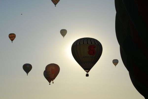
One of the participants to this meeting, who had shot 120 photos with his Nikon D200 digital camera, selected one of them, dated 5 August, on which appeared, in the upper left corner, among hot-air balloons, a quite singular unidentified object.
This case was reported by Mr. Christian Comtesse, who conducted a thorough on-site investigation , the final conclusions of which will be presented at the end.
Here is the photo – which we shall analyze – as it appeared, as well as a zoom on the unidentified object:

Data on the photographed scene
Depending on the circumstances and environment, one will try to identify elements appearing in the field – especially those which may be used for geometric or radiometric comparisons – and to assess their respective dimensions (size, distance from the camera, surface), in view of interpolating or extrapolating calculations, as well as characteristics in terms of luminance and color.
This may concern, for example, buildings, trees, relief, celestial bodies (sun, moon) or human beings.
The only visible elements of comparison in the scene photographed in Chambley are hot-air balloons. It was therefore important to make enquiries on the size of such objects.
Investigation on Internet taught us that a standard air-balloon has a volume in the order of 2500 m3, a height of 20 m and a diameter of 15 m.
Collection of technical data
Characteristics of the camera
All technical data of the camera as well as possible settings for the shot (focal length, focusing distance, exposure time) must be collected.
On the basis of a known camera model, it remains always possible to find out all characteristics, for if the operator himself does not have them to hand, the manufacturer can be consulted.
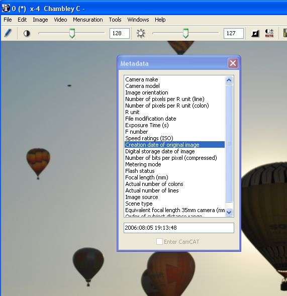
Besides, JPEG image files produced by digital cameras comprise, more and more systematically, metadata in the EXIF format, containing all required data on camera, date and settings. Access to original metadata, however, is only possible if the image file has not suffered any alteration.
Evaluation of the sharpness (or blurredness) of an object’s apparent shape may be essential in the frame of various distinct approaches.
- Movement blur: if, at shooting time, the object under analysis was moving and if this caused movement blur, it may be possible to quantify the object’s angular velocity at shooting time, using angular measurement of blurring and exposure time.
- Depth of field: if some blur may be related to the object being outside the depth of field, one may derive possible limits for the distance between object and camera (cf above).
- Atmospheric diffusion: independently from its consequences on apparent luminance of an object, atmospheric diffusion has degrading effects on sharpness of contours (MTF or Modulation Transfer Function), especially important if the object is remote. This feature is more or less visible, and thus measurable, according to weather conditions. In best cases (cloudy weather) it is possible to derive limits of possible distances by comparison with other objects in the scene, for which the distance from the camera at shooting time is known.
Color of an object
The object’s color may prove useful for analysis, as it provides (limited) information about the spectrum of light emitted, transmitted or reflected by that object. Besides, comparison with the dominant color of the scene may make it possible to bring out possible inconsistencies, that can be proof of a fake produced by image inlay.
Texture of an object
The object under analysis, if it covers a sufficient area in the photo, may display a texture, which depends on the material that constitutes or covers that object.
An image processing software will, in such a case, allow characterization of that texture, in view of comparison, if necessary, with a catalog of reference textures.
---------------------------------------------------------------------
Now, let's see practically how it works!
PRACTICAL ANALYSIS METHODOLOGY
This part sums up a standard sequence of actions to be taken in order to conduct analysis of an alleged UFO photo.
It will be illustrated, in the succeeding paragraphs, with the follow-up of a particular case in italics.
The file which we have chosen to illustrate – as far as possible – the different steps of photo analysis, concerns an incident which took place during the hot-air balloons competition Mondial Air Ballon 2007 which was organized, as every year, on the former military base of Chambley-les-Bussières (Meurthe-et-Moselle, France) in August 2007.
One of the participants to this meeting, who had shot 120 photos with his Nikon D200 digital camera, selected one of them, dated 5 August, on which appeared, in the upper left corner, among hot-air balloons, a quite singular unidentified object.
This case was reported by Mr. Christian Comtesse, who conducted a thorough on-site investigation , the final conclusions of which will be presented at the end.
Here is the photo – which we shall analyze – as it appeared, as well as a zoom on the unidentified object:
Data on the photographed scene
Depending on the circumstances and environment, one will try to identify elements appearing in the field – especially those which may be used for geometric or radiometric comparisons – and to assess their respective dimensions (size, distance from the camera, surface), in view of interpolating or extrapolating calculations, as well as characteristics in terms of luminance and color.
This may concern, for example, buildings, trees, relief, celestial bodies (sun, moon) or human beings.
The only visible elements of comparison in the scene photographed in Chambley are hot-air balloons. It was therefore important to make enquiries on the size of such objects.
Investigation on Internet taught us that a standard air-balloon has a volume in the order of 2500 m3, a height of 20 m and a diameter of 15 m.
Collection of technical data
Characteristics of the camera
All technical data of the camera as well as possible settings for the shot (focal length, focusing distance, exposure time) must be collected.
On the basis of a known camera model, it remains always possible to find out all characteristics, for if the operator himself does not have them to hand, the manufacturer can be consulted.
Besides, JPEG image files produced by digital cameras comprise, more and more systematically, metadata in the EXIF format, containing all required data on camera, date and settings. Access to original metadata, however, is only possible if the image file has not suffered any alteration.
Moreover, there exist a number of redundancies, and therefore means to regenerate pieces of data if they happen to be missing: for example, the real
dimensions of the photosensitive array may easily be derived from the focal length conversion factor, when this parameter is available.
The photo from Chambley has been obtained in its original format, which allowed recovery of EXIF metadata, on top of detailed technical information already provided by its author.
Camera settings
Parameters corresponding to settings possibly chosen by the operator should be collected from him as far as possible.
In addition, as already indicated, it is generally possible to find those data in metadata included in the image file.
In the particular case of focusing distance, if the operator remembers having shot while focusing on a given object, it is most useful to know or at least to estimate the real distance between that object and the camera, in view of accurate calculations on the depth of field.
Our photo sample was shot from the ground, with a Nikon D200 digital reflex camera focused to infinity, with an exposure time equal to 1/6400 sec.
Collecting image file and related metadata
As already explained, an image file should be collected in its original format, after it has undergone, as a maximum, nothing more than computer duplication, without any modification.
One will use different available media: preferably the memory stick of the camera (so as to be sure – in principle – that no transformation has been done outside that camera) or, if not, any other computer medium (e.g. USB stick, CD-Rom).
File generated by a digital camera
In order to access all the ancillary data comprised in the format, one will make use of specialized softwares. In the case – most of the time – of the EXIF format, there are numerous software solutions available to extract metadata, among which Exifer, GeoSetter, XnView, ACDSee, Imatch, PhotoME, and finally « IrfanView » (which, completed by the « EXIF » plug-in, has been recommended by the JPEG board).
My favorite software allows us simultaneously to display values of EXIF parameters present in an image, and to automatically exploit the same parameters for quick angular mensuration:
It can be done however, using maths formula, as we will see later....
Image photo-interpretation
Once an image file has been loaded onto his or her computer, the analyst may examine it and become familiar with it, with help of a specialized image viewing and processing software. By highlighting image details, an attempt will be made to establish parallels between this photo and already known cases, to detect possible clues and to establish some lines of thought, before initializing a deeper quantitative analysis.
The most useful image manipulation tools are also the most conventional ones: zoom, contrast enhancement, sharpness (high-pass) filtering, contour detection and the separation or enhancement of primary colors.
Many software tools may be used for such a work. The most well-known reference is Photoshop, an extremely powerful software in terms of interactive functionalities, essentially designed for photographers. A first approach is equally possible with simpler viewing tools, such as Irfanview.
The most appropriate solution is a CAPI tool, which, by definition, permits simultaneous interactive photo-interpretation (object of this paragraph) and quantitative analysis (the subject of the following paragraph), in a flexible and efficient approach. This is the case with the software I use in my analysis work.
Interactive manipulation of the photo from Chambley essentially consisted of zooming, taking advantage of the high resolution of the original document (10 megapixels).
At this point, one may imagine the object as possibly being a child’s balloon, or maybe a very big bird.
Quantitative image analysis
Geometric mensuration
Geometric mensuration on a digital photo relies on pixel localization in the image, which relate to the position of points of interest on the sensitive medium (the CCD array) and thus to the angular position of corresponding points in the scene.
A basic operation consists therefore in designating a point on the screen with a mouse, and in collecting its row and column coordinates. This can be done on the image, in full resolution (the image size then usually being larger than the screen, one will use the scroll boxes of the window to scroll it through), or making use of a zoom, which allows designation of a point of interest with better accuracy, sometimes to less than one pixel.
Comprehensive thread OP!
Related thread I authored a couple years ago:
A Method for Eliminating or Qualifying Known Objects Using Background Stars and Other Objects
www.abovetopsecret.com...
Related thread I authored a couple years ago:
A Method for Eliminating or Qualifying Known Objects Using Background Stars and Other Objects
www.abovetopsecret.com...
edit on 7-12-2012 by dainoyfb because: I added thread title.
reply to post by elevenaugust
How can we copy or save the info here?
By the way, I for one am impressed with your presentation.
njl51
How can we copy or save the info here?
By the way, I for one am impressed with your presentation.
njl51
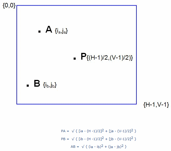
Coordinates of a point A in pixels are given in the form A [ia,ja], with:
ia : column number, from left to right on the screen, comprised between 0 and H-1
ja : row number, from top to bottom on the screen, comprised between 0 and V-1
H : total number of columns (thus of horizontal pixels)
V : total number of rows (thus of vertical pixels)
Coordinates of the center of the photo P being P [(H-1)/2,(V-1)/2], distances in pixels between P and two points A and B are:
Those distances in pixels may then be converted into physical distances on the photosensitive medium, simply by applying the rule of three, if real physical dimensions of that medium are available.
Dimensions of the photosensitive array may be directly obtained with the technical characteristics of the camera, or inferred from the focal length conversion factor (if it is provided), either with technical characteristics, or with EXIF metadata associated with the photo (depending on manufacturers).
One should keep in mind that this conversion factor is to be applied to the diagonal of the rectangular (or square) surface of the sensor. Generally, it corresponds to the ratio of the diagonal of a 24x36 mm standard silver format – i.e. 43,3 mm – to the diagonal of the CCD array of the digital camera.
From the physical dimensions on the sensitive medium and from the focal length, one may derive the calculation of angular dimensions. Then, possible estimates of absolute dimensions may be obtained (cf above).
Regarding the estimation of distance between the object under study and the camera, a few approaches (cf above) require radiometric measures or sharpness estimates. One should then address respectively the two following sections.
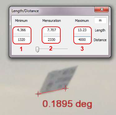
The very relevant angular size mensuration on the photo from Chambley concerns the largest apparent dimension of the unidentified object (we shall refer to its « length ») and the hot-air balloons (we shall concentrate on the horizontal diameters of two of them).
The software permits direct calculation of such angular sizes in a few clicks, taking automatically advantage of available EXIF metadata. For the sake of illustration however, we shall go through the calculations step by step.
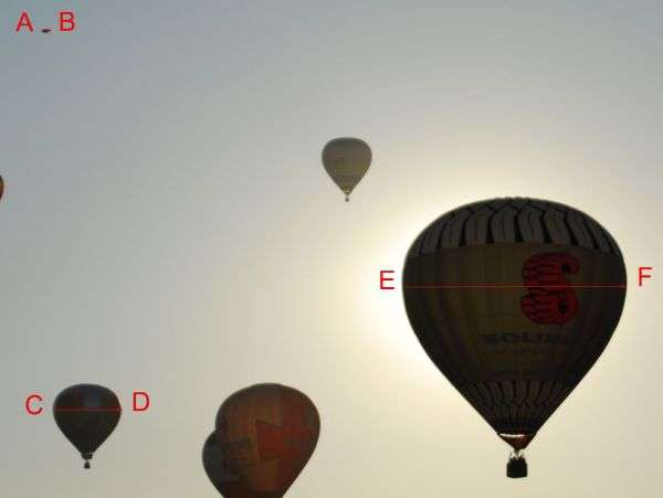
First, we interactively collect the coordinates of the 6 pixels designated in the image below (image size: 3872 columns, 2592 rows) :
[align=center]Extremities of the unidentified object : A [550,371] B [582,368][/align]
[align=center]Side extremities of balloon 1 : C [591,1753] D [841,1753][/align]
[align=center]Side extremities of balloon 2 : E [1864,1288] F [2689,1288][/align]
The calculation of angular size of the unidentified object is performed as follows, referring to above-mentioned formulas (where P is the center of the photo):
[align=center]PA = √ [ (550 – 1935,5)sqr + (371 – 1295,5)sqr ] = 1666 pixels[/align]
[align=center]PB = √ [ (582 – 1935,5)sqr + (368 – 1295,5)sqr ] = 1641 pixels[/align]
[align=center]AB = √ [ (550 – 582)sqr + (371 – 368)sqr ] = 32 pixels[/align]
The focal length being equal to 80 mm (EXIF data), and the focal length conversion factor being equal to 1,5 (technical data of the camera), we are back to the case of a 24x36 mm camera with a focal length f = 120 mm (other EXIF piece of data called « Equivalent focal length 35mm camera »).
In that frame (24x36 mm), the effective dimension of one pixel equals:
thus:
Applying the generalized Pythagoras’ theorem, we may calculate the angular size of the unidentified object:
[align=center]δ object = arccos [(2x120sqr+15,46sqr+15,23sqr–0,30sqr) / 2√[(120sqr+15,46sqr)(120sqr+15,23sqr)]][/align]
In the same way, we calculate the angular size (horizontal diameter) of both reference balloons:
ia : column number, from left to right on the screen, comprised between 0 and H-1
ja : row number, from top to bottom on the screen, comprised between 0 and V-1
H : total number of columns (thus of horizontal pixels)
V : total number of rows (thus of vertical pixels)
Coordinates of the center of the photo P being P [(H-1)/2,(V-1)/2], distances in pixels between P and two points A and B are:
Those distances in pixels may then be converted into physical distances on the photosensitive medium, simply by applying the rule of three, if real physical dimensions of that medium are available.
Dimensions of the photosensitive array may be directly obtained with the technical characteristics of the camera, or inferred from the focal length conversion factor (if it is provided), either with technical characteristics, or with EXIF metadata associated with the photo (depending on manufacturers).
One should keep in mind that this conversion factor is to be applied to the diagonal of the rectangular (or square) surface of the sensor. Generally, it corresponds to the ratio of the diagonal of a 24x36 mm standard silver format – i.e. 43,3 mm – to the diagonal of the CCD array of the digital camera.
From the physical dimensions on the sensitive medium and from the focal length, one may derive the calculation of angular dimensions. Then, possible estimates of absolute dimensions may be obtained (cf above).
Regarding the estimation of distance between the object under study and the camera, a few approaches (cf above) require radiometric measures or sharpness estimates. One should then address respectively the two following sections.
The very relevant angular size mensuration on the photo from Chambley concerns the largest apparent dimension of the unidentified object (we shall refer to its « length ») and the hot-air balloons (we shall concentrate on the horizontal diameters of two of them).
The software permits direct calculation of such angular sizes in a few clicks, taking automatically advantage of available EXIF metadata. For the sake of illustration however, we shall go through the calculations step by step.
First, we interactively collect the coordinates of the 6 pixels designated in the image below (image size: 3872 columns, 2592 rows) :
[align=center]Extremities of the unidentified object : A [550,371] B [582,368][/align]
[align=center]Side extremities of balloon 1 : C [591,1753] D [841,1753][/align]
[align=center]Side extremities of balloon 2 : E [1864,1288] F [2689,1288][/align]
The calculation of angular size of the unidentified object is performed as follows, referring to above-mentioned formulas (where P is the center of the photo):
[align=center]PA = √ [ (550 – 1935,5)sqr + (371 – 1295,5)sqr ] = 1666 pixels[/align]
[align=center]PB = √ [ (582 – 1935,5)sqr + (368 – 1295,5)sqr ] = 1641 pixels[/align]
[align=center]AB = √ [ (550 – 582)sqr + (371 – 368)sqr ] = 32 pixels[/align]
The focal length being equal to 80 mm (EXIF data), and the focal length conversion factor being equal to 1,5 (technical data of the camera), we are back to the case of a 24x36 mm camera with a focal length f = 120 mm (other EXIF piece of data called « Equivalent focal length 35mm camera »).
In that frame (24x36 mm), the effective dimension of one pixel equals:
36/3871 ≈ 24/2591 ≈ 0,00928 mm
thus:
a = PA = 15,46 mm
b = PB = 15,23 mm
d = AB = 0,30 mm
Applying the generalized Pythagoras’ theorem, we may calculate the angular size of the unidentified object:
[align=center]δ object = arccos [(2x120sqr+15,46sqr+15,23sqr–0,30sqr) / 2√[(120sqr+15,46sqr)(120sqr+15,23sqr)]][/align]
δ object = 0,14 °
In the same way, we calculate the angular size (horizontal diameter) of both reference balloons:
δ balloon1 = 1,10 °
δ balloon2 = 3,65 °
Originally posted by dainoyfb
Comprehensive thread OP!
Related thread I authored a couple years ago:
A Method for Eliminating or Qualifying Known Objects Using Background Stars and Other Objects
www.abovetopsecret.com...
edit on 7-12-2012 by dainoyfb because: I added thread title.
Thank you!
I'll look at your thread ASAP, many thanks for the link
Originally posted by njl51
reply to post by elevenaugust
How can we copy or save the info here?
By the way, I for one am impressed with your presentation.
njl51
Thanks! You still can quote my posts whenever you want. Feel free to PM me for more informations!
Luminance estimation
Directly measurable data which quantify light collected by a given pixel of a digital photo are gray levels (in black and white) or respective brightness levels in the 3 primary colors (red, green, blue). Those values represent the apparent luminance of corresponding points in the scene, with certain limitations.
It is only possible, in this domain, to produce estimates and to sort objects according to increasing or decreasing values of their apparent luminance. Nevertheless, this may be enough to perform a rough interpolation and to estimate a range of possible distances between the object and the lens.
One will use, for this type of mensuration, an image viewing or processing software providing levels of a selected pixel on the screen through a mouse, or statistics on level values in a given image area graphically selected on the screen, or a plot of level variation along a designated vector (a radiometric cross-section).
Here are examples to illustrate these types of mensuration, using our software:
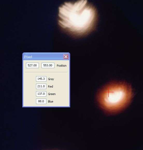
To the cursor position (red cross) correspond the coordinates (position) of the selected pixel, as well as its RGB levels (red, green, blue) and gray level (average of the 3).
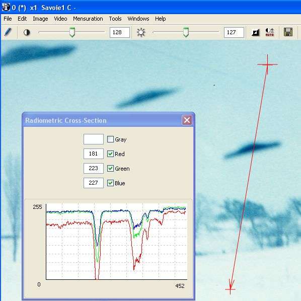
To the vector drawn on the right of the image (red arrow) correspond the plot of the radiometric cross-section showing variations of the levels (representing apparent luminance), displayed in the window.
Our photo sample was shot against the sunlight and we may consider that the darkest parts of the objects of the scene were submitted to variations of their apparent luminance mostly due to atmospheric diffusion. Consequently, we shall concentrate on the dark part of the unidentified object, as well as that of both reference balloons.
In a quite empirical approach, we shall content ourselves with noting down the darkest pixel value in each of these three areas, using the tool dedicated to the analysis of the radiometry of pixels within in a closed surface (here a red circle)..
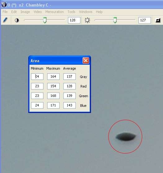
Dark level object = 24
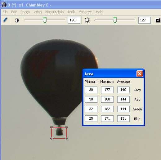
The same for both reference balloons’ baskets.
Balloon 1 :
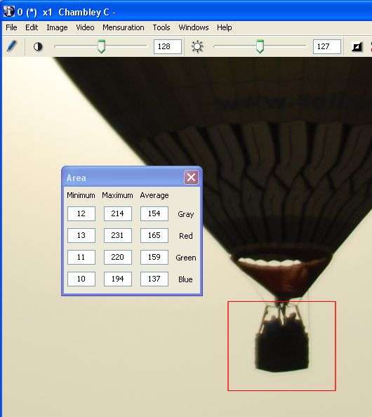
Balloon 2:
Dark level balloon1 = 30
Dark level balloon2 = 12
Assuming – which is highly probable – that the object and both reference baskets are really dark, we may conclude that the distance of the object from the camera was somewhere between that of balloon 1 and that of balloon 2. In fact, those distances may be estimated, if we assume that both balloons have a standard diameter Ф = 15 m:
Through linear interpolation on the darkest pixel values (an empirical approach), we obtain an estimate of the distance to the unidentified object:
From which we may derive an estimate of its actual length:
Length object = 2 x 300 tan (0,14°/2) i.e.:
Taking into account uncertainties and calculation approximations, we can conservatively conclude that the length of the object – if it was actually dark – was somewhere between 50 cm and 1 m.
Directly measurable data which quantify light collected by a given pixel of a digital photo are gray levels (in black and white) or respective brightness levels in the 3 primary colors (red, green, blue). Those values represent the apparent luminance of corresponding points in the scene, with certain limitations.
It is only possible, in this domain, to produce estimates and to sort objects according to increasing or decreasing values of their apparent luminance. Nevertheless, this may be enough to perform a rough interpolation and to estimate a range of possible distances between the object and the lens.
One will use, for this type of mensuration, an image viewing or processing software providing levels of a selected pixel on the screen through a mouse, or statistics on level values in a given image area graphically selected on the screen, or a plot of level variation along a designated vector (a radiometric cross-section).
Here are examples to illustrate these types of mensuration, using our software:
To the cursor position (red cross) correspond the coordinates (position) of the selected pixel, as well as its RGB levels (red, green, blue) and gray level (average of the 3).
To the vector drawn on the right of the image (red arrow) correspond the plot of the radiometric cross-section showing variations of the levels (representing apparent luminance), displayed in the window.
Our photo sample was shot against the sunlight and we may consider that the darkest parts of the objects of the scene were submitted to variations of their apparent luminance mostly due to atmospheric diffusion. Consequently, we shall concentrate on the dark part of the unidentified object, as well as that of both reference balloons.
In a quite empirical approach, we shall content ourselves with noting down the darkest pixel value in each of these three areas, using the tool dedicated to the analysis of the radiometry of pixels within in a closed surface (here a red circle)..
Dark level object = 24
The same for both reference balloons’ baskets.
Balloon 1 :
Balloon 2:
Dark level balloon1 = 30
Dark level balloon2 = 12
Assuming – which is highly probable – that the object and both reference baskets are really dark, we may conclude that the distance of the object from the camera was somewhere between that of balloon 1 and that of balloon 2. In fact, those distances may be estimated, if we assume that both balloons have a standard diameter Ф = 15 m:
Distance balloon1 = (Ф/2) / tan (δ ballon1 / 2) i.e.: Distance balloon1 = 391 m
Distance balloon2 = (Ф/2) / tan (δ balloon2 / 2) i.e.: Distance balloon2 = 118 m
Through linear interpolation on the darkest pixel values (an empirical approach), we obtain an estimate of the distance to the unidentified object:
Distance object = 300 m
From which we may derive an estimate of its actual length:
Length object = 2 x 300 tan (0,14°/2) i.e.:
Length object = 0,73 m
Taking into account uncertainties and calculation approximations, we can conservatively conclude that the length of the object – if it was actually dark – was somewhere between 50 cm and 1 m.
Sharpness estimation (FTM)
Sharpness estimation of the contours of an object, apart from the case of a movement blur (which must be analyzed case by case), may be used to assess the distance of that object, following two possible approaches.
On one hand, if the object was outside the depth of field, it appeared inevitably more blurred on the photo than objects located inside the depth of field. This is particularly the case for very small objects very close to the lens, especially if they are illuminated by the flash (see numerous photographs displaying « orbs »).
On the other hand, it is sometimes observed that, within the depth of field, the apparent sharpness of an object deteriorates progressively as the object moves away, because of atmospheric diffusion. The crossed atmosphere layer is characterized by its MTF, and behaves like a low-pass filter in the spatial frequency domain, this phenomenon being more or less measurable depending on weather conditions. Comparison of contours of the object under study and of other objects located at known or estimated distances from the camera then allows us to narrow the range of possible distance of the object.
The only simple empirical way to estimate the sharpness of a contour is to plot a radiometric cross-section (of the same nature as a densitometric cross-section in silver photography) perpendicular to that contour. Indeed, the spatial frequency spectrum is linked through Fourier transform, in the bidimensional image space, to the impulse response (image of a point light source), which in turn may be linked in a monodimensional form by the response, in a given direction, to the « step function » made of the discontinuity of an object’s contour.
In practice, the more the gray level transition curve, on either side of a contour, spreads over a large width (in other words: the shallower the transition slope), the more the image has been degraded by the MTF of the atmosphere, and therefore the farther away was the object (through a commensurately thicker atmospheric layer), all other things being equal.
Here again, it is often only possible to make an empirical interpolation between the « contour responses » of several objects in the scene, allowing to « sort » them by increasing distances from the camera.

Estimate of radiometric slope along a designated vector, perpendicular to the contour of the object being analyzed : the transition slope is here estimated to 7,33 levels/pixel (transition from 10% to 90% over 19,7 pixels).
Unfortunately, weather conditions in Chambley, where our sample photo was taken, with an excellent visibility, do not allow detection of any degradation of the sharpness of contours by atmospheric diffusion (the maximum slopes of radiometric cross-sections perpendicular to the respective contours of the unidentified object and of both reference balloons are of the same order of magnitude).
--------------------------------------------------------------------------------------------
Final report of the Chambley case, from Mr. Comtesse, in French
Sharpness estimation of the contours of an object, apart from the case of a movement blur (which must be analyzed case by case), may be used to assess the distance of that object, following two possible approaches.
On one hand, if the object was outside the depth of field, it appeared inevitably more blurred on the photo than objects located inside the depth of field. This is particularly the case for very small objects very close to the lens, especially if they are illuminated by the flash (see numerous photographs displaying « orbs »).
On the other hand, it is sometimes observed that, within the depth of field, the apparent sharpness of an object deteriorates progressively as the object moves away, because of atmospheric diffusion. The crossed atmosphere layer is characterized by its MTF, and behaves like a low-pass filter in the spatial frequency domain, this phenomenon being more or less measurable depending on weather conditions. Comparison of contours of the object under study and of other objects located at known or estimated distances from the camera then allows us to narrow the range of possible distance of the object.
The only simple empirical way to estimate the sharpness of a contour is to plot a radiometric cross-section (of the same nature as a densitometric cross-section in silver photography) perpendicular to that contour. Indeed, the spatial frequency spectrum is linked through Fourier transform, in the bidimensional image space, to the impulse response (image of a point light source), which in turn may be linked in a monodimensional form by the response, in a given direction, to the « step function » made of the discontinuity of an object’s contour.
In practice, the more the gray level transition curve, on either side of a contour, spreads over a large width (in other words: the shallower the transition slope), the more the image has been degraded by the MTF of the atmosphere, and therefore the farther away was the object (through a commensurately thicker atmospheric layer), all other things being equal.
Here again, it is often only possible to make an empirical interpolation between the « contour responses » of several objects in the scene, allowing to « sort » them by increasing distances from the camera.
Estimate of radiometric slope along a designated vector, perpendicular to the contour of the object being analyzed : the transition slope is here estimated to 7,33 levels/pixel (transition from 10% to 90% over 19,7 pixels).
Unfortunately, weather conditions in Chambley, where our sample photo was taken, with an excellent visibility, do not allow detection of any degradation of the sharpness of contours by atmospheric diffusion (the maximum slopes of radiometric cross-sections perpendicular to the respective contours of the unidentified object and of both reference balloons are of the same order of magnitude).
--------------------------------------------------------------------------------------------
Final report of the Chambley case, from Mr. Comtesse, in French
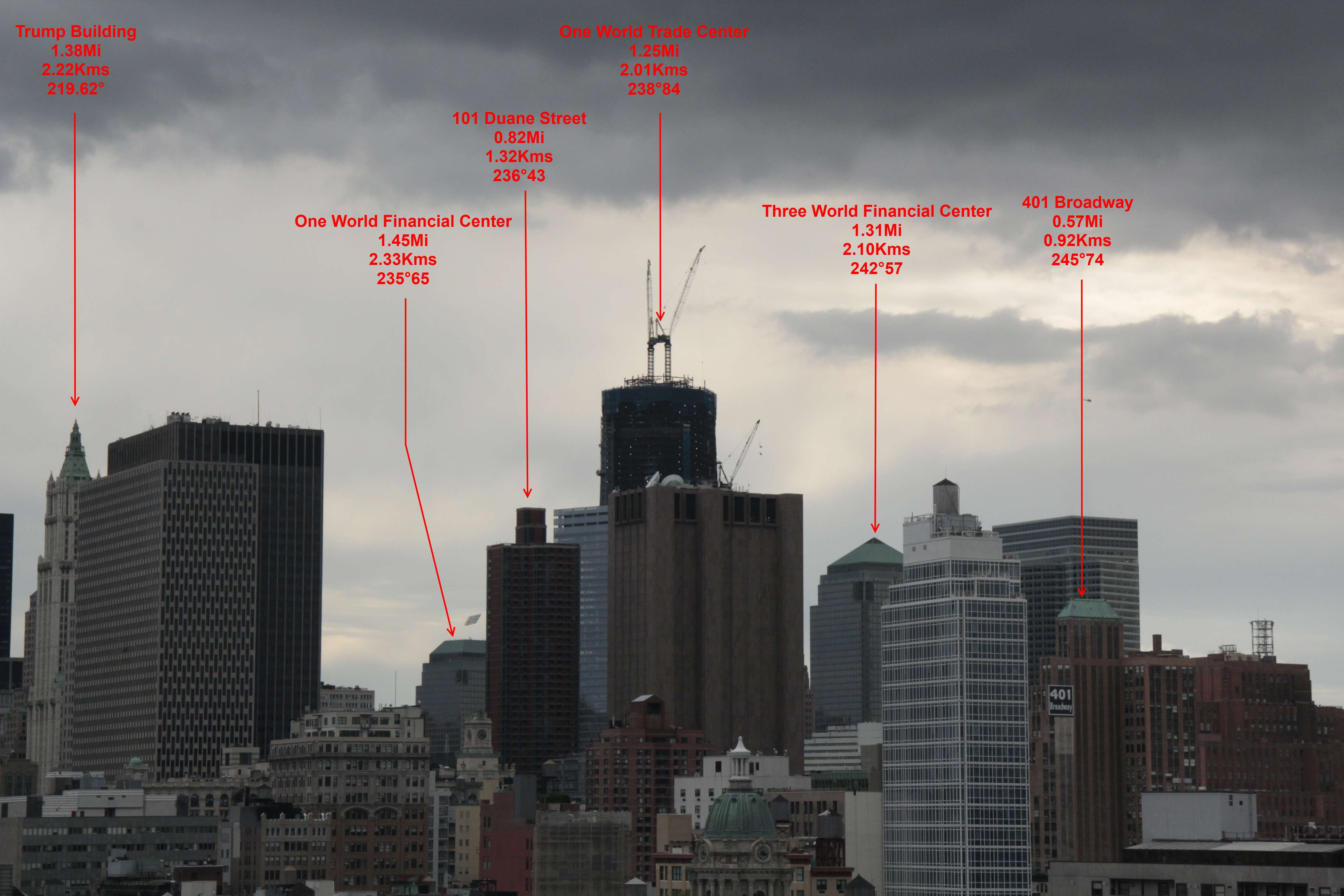
Here are two other examples in which I used this methodology:
- The Cecconi case photos - 1979

- The New-York case - 2011
- The Cecconi case photos - 1979
- The New-York case - 2011
new topics
-
Maestro Benedetto
Literature: 1 hours ago -
Is AI Better Than the Hollywood Elite?
Movies: 1 hours ago -
Las Vegas UFO Spotting Teen Traumatized by Demon Creature in Backyard
Aliens and UFOs: 4 hours ago -
2024 Pigeon Forge Rod Run - On the Strip (Video made for you)
Automotive Discussion: 5 hours ago -
Gaza Terrorists Attack US Humanitarian Pier During Construction
Middle East Issues: 5 hours ago -
The functionality of boldening and italics is clunky and no post char limit warning?
ATS Freshman's Forum: 6 hours ago -
Meadows, Giuliani Among 11 Indicted in Arizona in Latest 2020 Election Subversion Case
Mainstream News: 7 hours ago -
Massachusetts Drag Queen Leads Young Kids in Free Palestine Chant
Social Issues and Civil Unrest: 7 hours ago -
Weinstein's conviction overturned
Mainstream News: 9 hours ago -
Supreme Court Oral Arguments 4.25.2024 - Are PRESIDENTS IMMUNE From Later Being Prosecuted.
Above Politics: 10 hours ago
top topics
-
Krystalnacht on today's most elite Universities?
Social Issues and Civil Unrest: 10 hours ago, 9 flags -
Supreme Court Oral Arguments 4.25.2024 - Are PRESIDENTS IMMUNE From Later Being Prosecuted.
Above Politics: 10 hours ago, 8 flags -
University of Texas Instantly Shuts Down Anti Israel Protests
Education and Media: 13 hours ago, 7 flags -
Weinstein's conviction overturned
Mainstream News: 9 hours ago, 7 flags -
Gaza Terrorists Attack US Humanitarian Pier During Construction
Middle East Issues: 5 hours ago, 7 flags -
Massachusetts Drag Queen Leads Young Kids in Free Palestine Chant
Social Issues and Civil Unrest: 7 hours ago, 6 flags -
Meadows, Giuliani Among 11 Indicted in Arizona in Latest 2020 Election Subversion Case
Mainstream News: 7 hours ago, 5 flags -
Las Vegas UFO Spotting Teen Traumatized by Demon Creature in Backyard
Aliens and UFOs: 4 hours ago, 4 flags -
2024 Pigeon Forge Rod Run - On the Strip (Video made for you)
Automotive Discussion: 5 hours ago, 2 flags -
Any one suspicious of fever promotions events, major investor Goldman Sachs card only.
The Gray Area: 15 hours ago, 2 flags
active topics
-
VP's Secret Service agent brawls with other agents at Andrews
Mainstream News • 61 • : Scratchpost -
University of Texas Instantly Shuts Down Anti Israel Protests
Education and Media • 228 • : cherokeetroy -
SETI chief says US has no evidence for alien technology. 'And we never have'
Aliens and UFOs • 72 • : yuppa -
My Poor Avocado Plant.
General Chit Chat • 77 • : JonnyC555 -
New whistleblower Jason Sands speaks on Twitter Spaces last night.
Aliens and UFOs • 61 • : Ophiuchus1 -
Is AI Better Than the Hollywood Elite?
Movies • 2 • : 5thHead -
Gaza Terrorists Attack US Humanitarian Pier During Construction
Middle East Issues • 25 • : CarlLaFong -
Mood Music Part VI
Music • 3102 • : Hellmutt -
Las Vegas UFO Spotting Teen Traumatized by Demon Creature in Backyard
Aliens and UFOs • 9 • : Ophiuchus1 -
British TV Presenter Refuses To Use Guest's Preferred Pronouns
Education and Media • 164 • : Annee
7